Predicting House Prices Using Advanced Regression Model
The American Dream is a phrase to describe a pursuit of various opportunities that are equally available to Americans, that allow them to reach for their highest life aspirations and goals. The core components of American Dream, according to Rank(2014), are the freedom to pursue one's interests and passions in life. Secondly, the importance of economic security and well-being. Lastly, the importance of having hope and optimism with respect to seeing process in one's life. These three beliefs constitute the common social goal that motivate Americans to uphold one another, and make an impact on other societies to lead by example. Even in this day and age where we have significantly polarizing political views, this idealism seems to be the sole resonating motivator that binds Americans together.
However, there are many criticisms that the contemporary interpretation of the phrase 'American Dream' become more of a reminder of a dream of individual success and wealth. According to Diamond(2018), the phrase meant the opposite of what it does now a century ago, and was repurposed by each generation. The original dream was not about the prospect of one's accomplishments or affluence, but was about the hope of equality, justice and democracy for the nation. It was not until the Cold War that the phrase became an argument for a consumer capitalist version of democracy, and have not been argued otherwise since the 1950's. Consequently, this argument has now become widely-accepted understanding of the phrase of this generation.
Nevertheless, the ideology goes far beyond its understanding of the phrase. The primary focus is always been more towards the abundance of equal opportunities available to Americans to achieve their individual dream and increase their quality of living. These opportunities might include accessibility to affordable healthcare, higher education, higher-paying quality jobs, and many more. Though the definition of quality of living may be highly subjective, these opportunities will undoubtably be a collection of factors that play a major role in healthy living, financial security, and job satisfaction. Ultimately, at the heart of the American Dream is always been about the desire to own a home as a reward to have kept dreaming the dream, and to inspire the next generation of American dreamers.
Source:
Rank, Mark. “What Is the American Dream?” Oxford University Press , 1 July 2014,
blog.oup.com/2014/07/questioning-american-dream/.
Diamond, Anna. “The Original Meanings of the ‘American Dream’ and ‘America First’ Were Starkly Different From How We Use Them Today.” Smithsonian Magazine , Oct. 2018.
smithsonianmag.com/history/behold-america-american-dream-slogan-book-sarah-churchwell-180970311/.
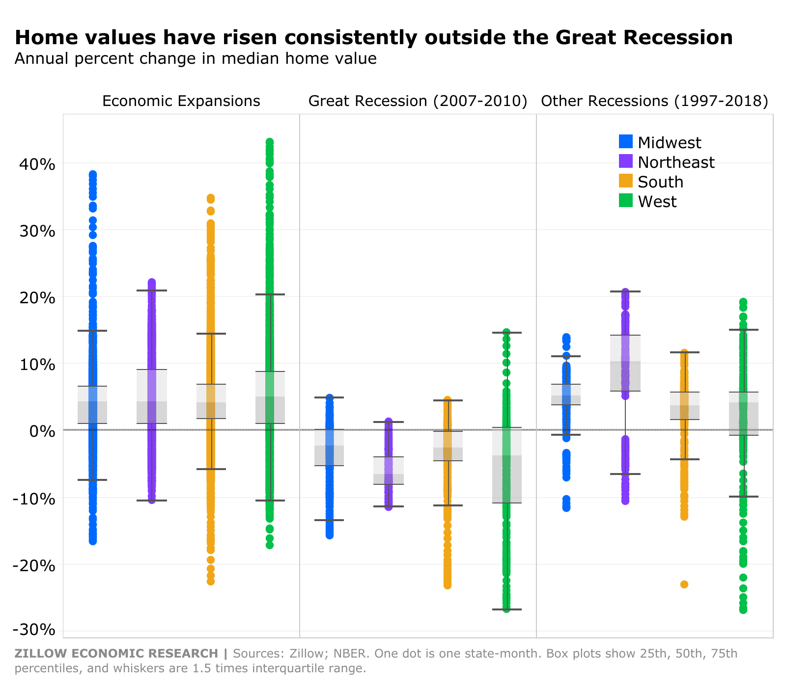
Source: Zillow Research
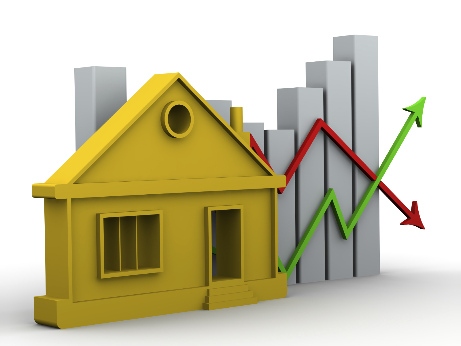
Homeownership became an essential product of the American Dream that is now synonymous with economic security and middle-class status. Buying a home may be the largest financial investment many will make so it is advised that a potential buyer is financially ready to make the purchase. Becoming a homeowner is not only a big financial commitment, but also a testament to make the best effort to maintain the property to keep the financial value of their house and the family's socioeconomic status. This is also the moment that has been long awaited for many families. It is expected for them to feel compelled to consider the perfect property within their budget that can encompass many aspects of their lives. Consequently, it is only natural that the home buying process that can capture these societal values as well as their needs and wants feels overwhelming.
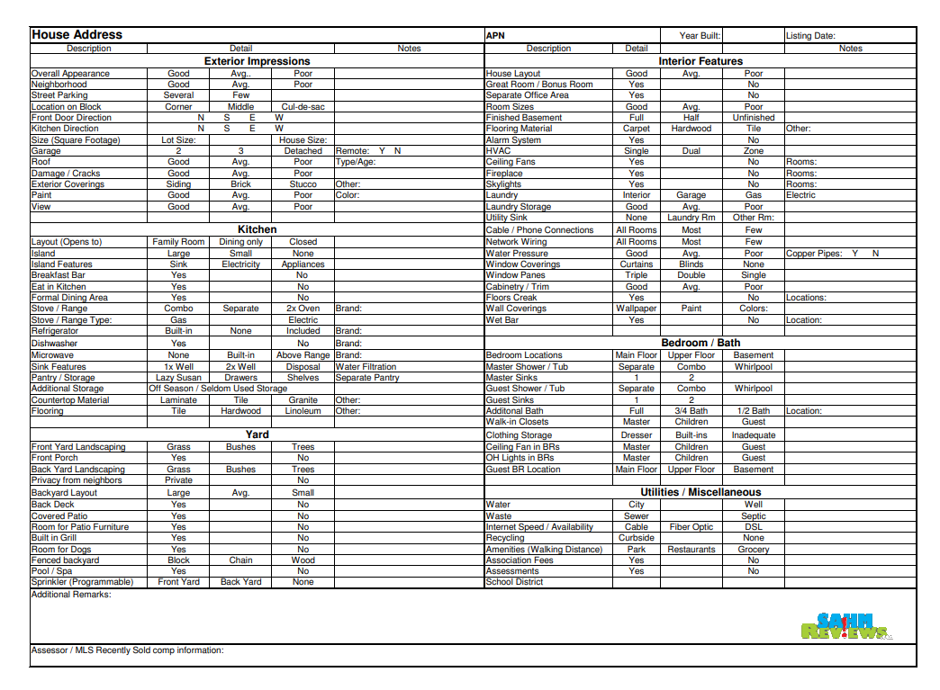
Fortunately, one of many ways to cope when faced with such enormous life challenge is to follow a home buying checklist. A typical home buying checklist, much like the one depicted above, is a handy tool that breaks down the home-buying process step-by-step. It lays out a systematic approach to check for every feature of the house in detail to determine its attractiveness to the buyer. This will help to make the process feel manageable as well as predictable. In this study, we will attempt to put ourselves in the shoes of a potential home buyer in a similar situation. We will study a number of house features of various properties in a neighborhood of Iowa in an attempt to predict the affordability using a statistical learning model.
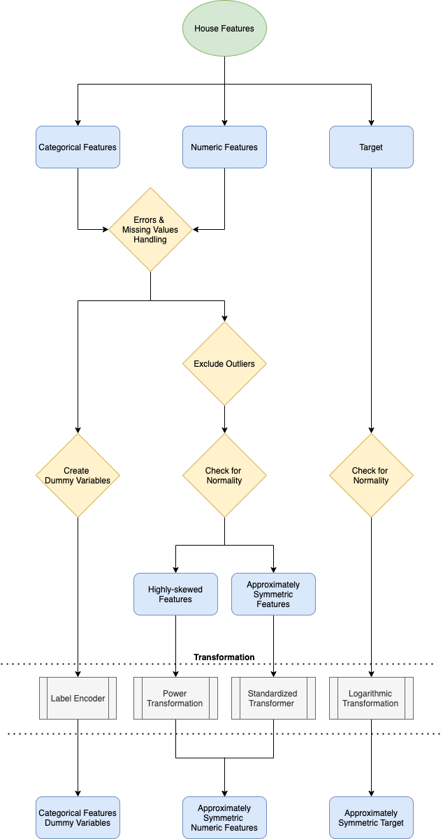
Feature Engineering Flow Chart
Approach
We begin our process by dissecting the dataset into two major parts. These parts are categorical features and numeric features. Categorical features explain the quality and type variables. Numeric features convey the quantity and area variables. Moreover, we can split up the numeric variables further by initiating an exploratory data analysis. By performing a check for normality of our variables, we can break up our numeric variables into two smaller components separated by their level of skewness. Finally, we will be transforming our distribution of numeric variables to be approximately symmetrical to minimize the variance in our predictions, which will be explained further in detail below.
Assumption
We typically don't describe our dream house with the height of the basement ceiling or the proximity to an east-west railroad. But, the dataset that we will going to be exploring proves that there are much more influences to price negotiations than the number of bedrooms or a white-picket fence. With 79 explanatory variables describing (almost) every aspect of residential homes in Ames, Iowa, we are challenged to predict the final price of each home. These variables focus primary on the quality and quantity of many physical attributes of the property. They help answer exactly the type of information that a typical home buyer would want to know about a potential property such as the year it was built, the square feet of living space, and the number of bedrooms. In this study, we will not be including any other information besides the features described above to fit our prediction model. In addition, the information about any other neighborhoods is not included in the dataset. Our focus is to predict sale prices of properties with solely on different attributes.
Goal
The goal for this study is to predict the sale prices of properties in Ames, Iowa by training a statitical model using various types of information about the physical attributes of each property.
Gradient Boosting Regression Model Diagram
Walkthrough
∘ Define Data Path
∘ Import Libraries
∘ Define Exploratory Data Analysis Functions
∘ Define ML Model Functions
∘ Define Plotting Functions
∘ Perform Data Acquisition and Preparation
1. Define DataFrames, Features and Target
Acquire Train Dataset and Transform DataFrame
∘ Retrieve Original Sample Train DataFrame
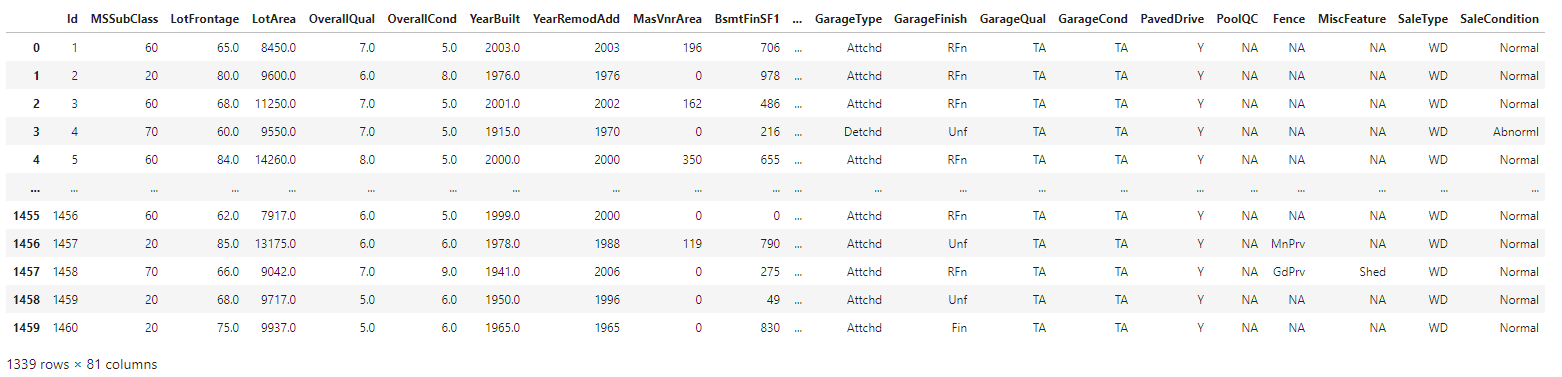
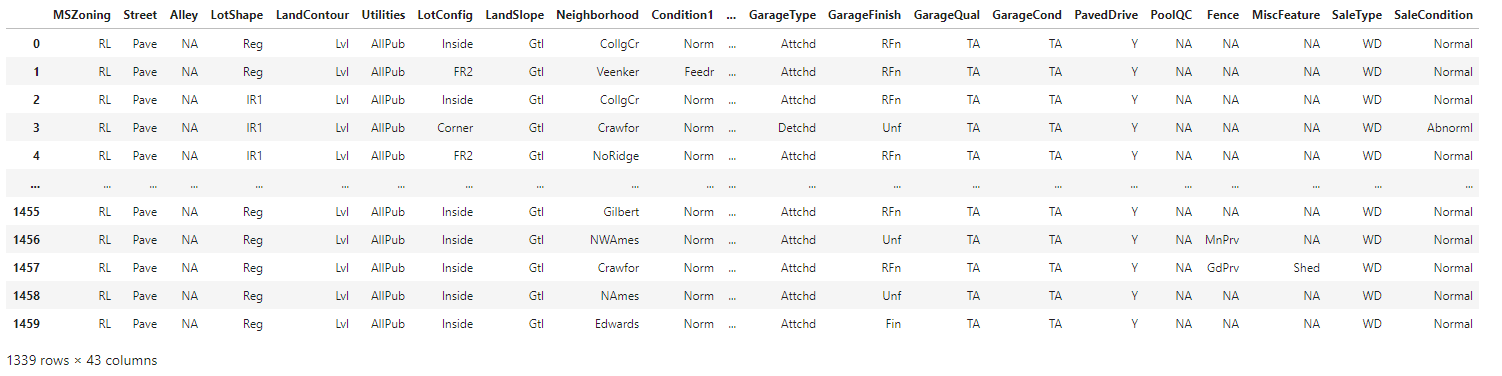
∘ Display Categorical Features in Train DataFrame
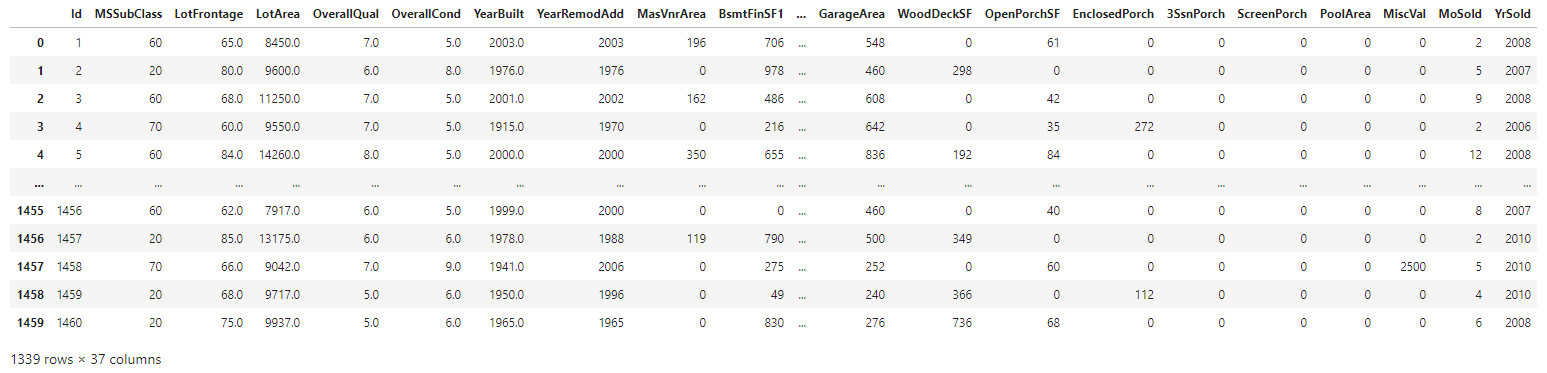
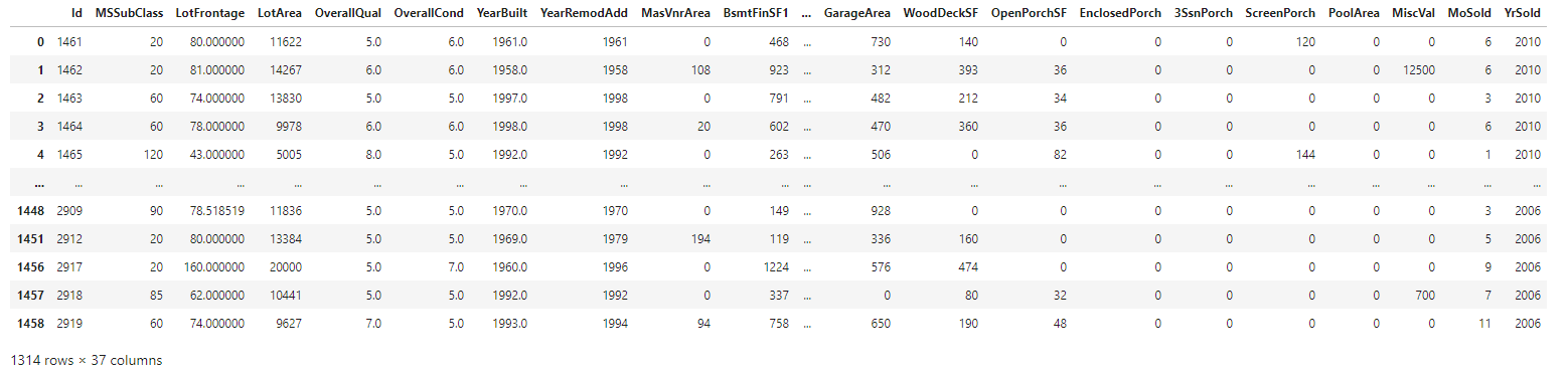
∘ Display Numerical Features in Train DataFrame
Retrieve Original Sample Test DataFrame
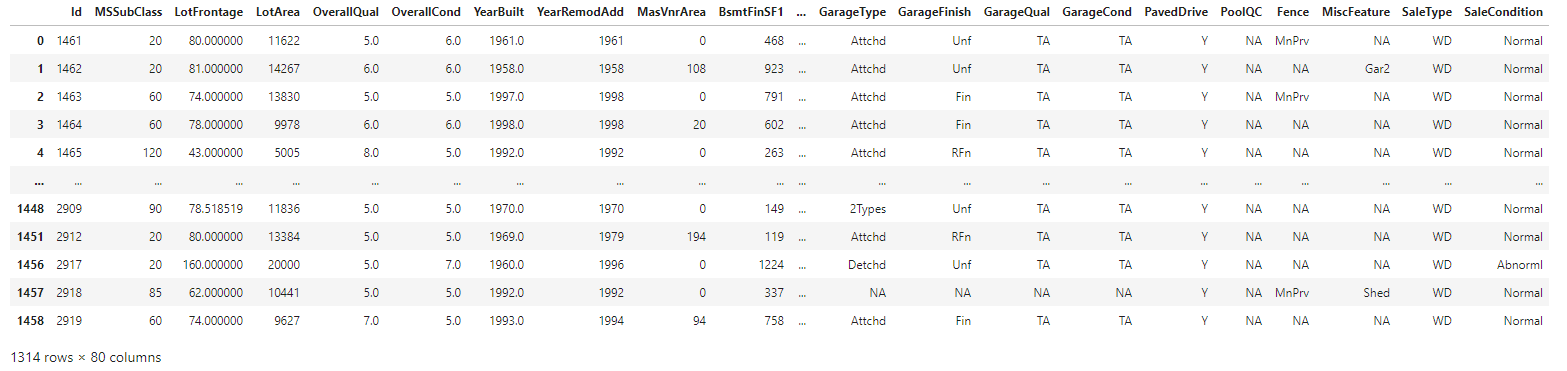
∘ Retrieve Original Sample Test DataFrame
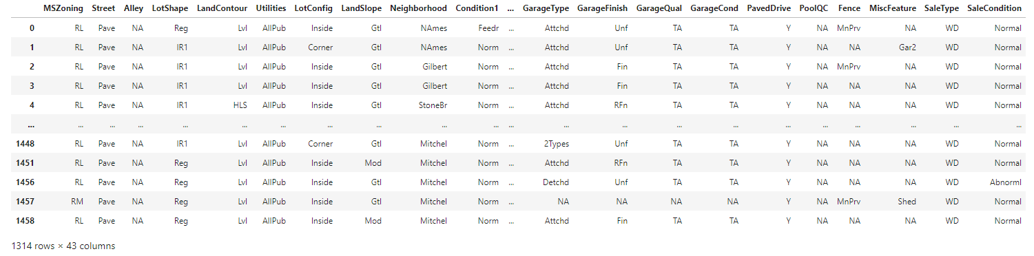
∘ Display Categorical Features in Test DataFrame
∘ Display Numerical Features in Test DataFrame
Files
Columns
∘ Handling Missing Values
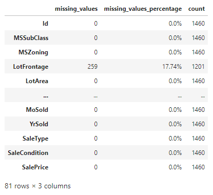
∘ Dispaly Missing Values DataFrame
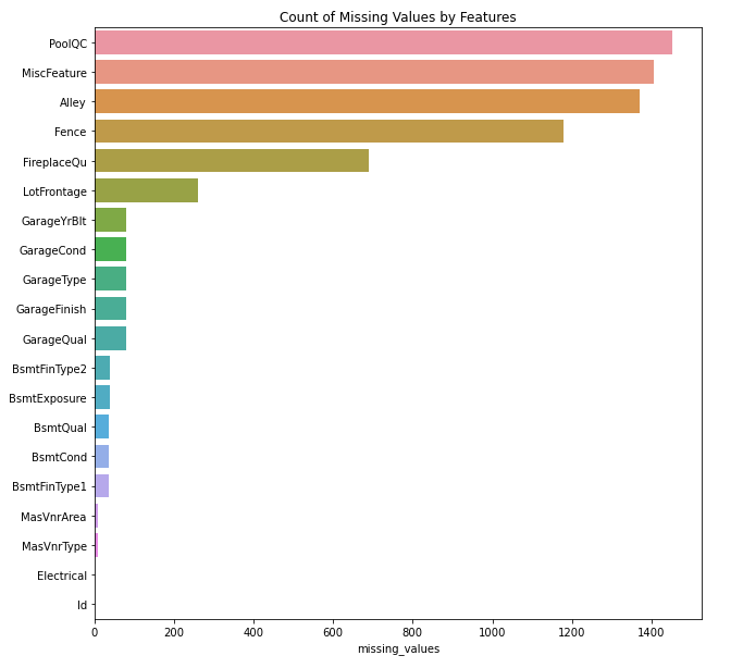
Plotting Top 20 Columns with Most Number of Missing Values
∘ Display Missing Values Handling Function
Our feature engineering begins with checking for missing values in our data or information that is not consistent. For example, we have a significant number of values information missing about the quality of swimming pool included in a number of properties. To determine its quality, we first have to make sure that the property includes a pool. By checking the information containing the square footage of the pool, we may be able to extract a key detail about whether the property includes a swimming pool or not. If the information about the area of the pool is not there, or the value is zero, we can safely assume that the property does not include a pool. On the other hand, if we determined that the property does include a swimming pool, and the value for the area is greater than zero, we will handle our missing information about the pool quality as below average to make sure that we do not exaggerate or underrate the property's attribute for the benefit of the doubt. By exploring different type and aspect of information regarding the same physical attribute of the property, we will be able to manage any inconsistency in our data. With this rationale, we will try to tackle rest of the features with any missing values.
∘ Exploring Numeric Features
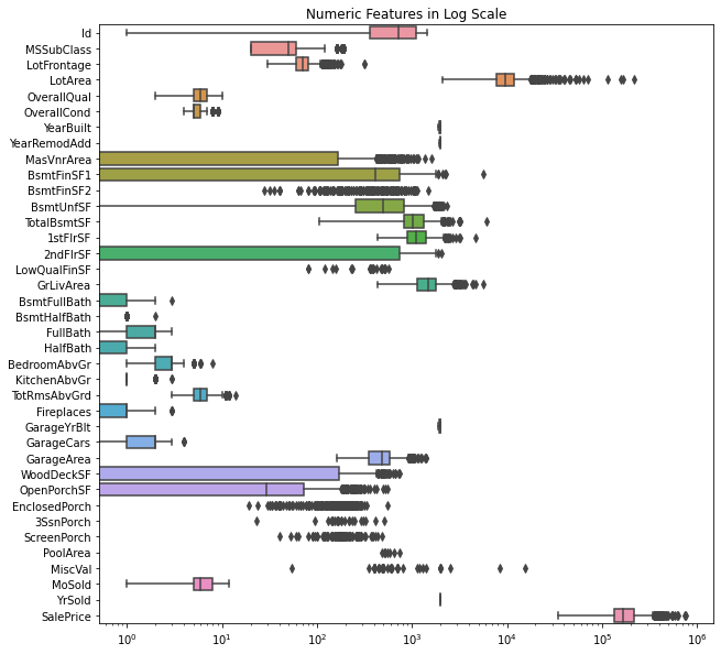
Plotting Distribution of Numeric Features
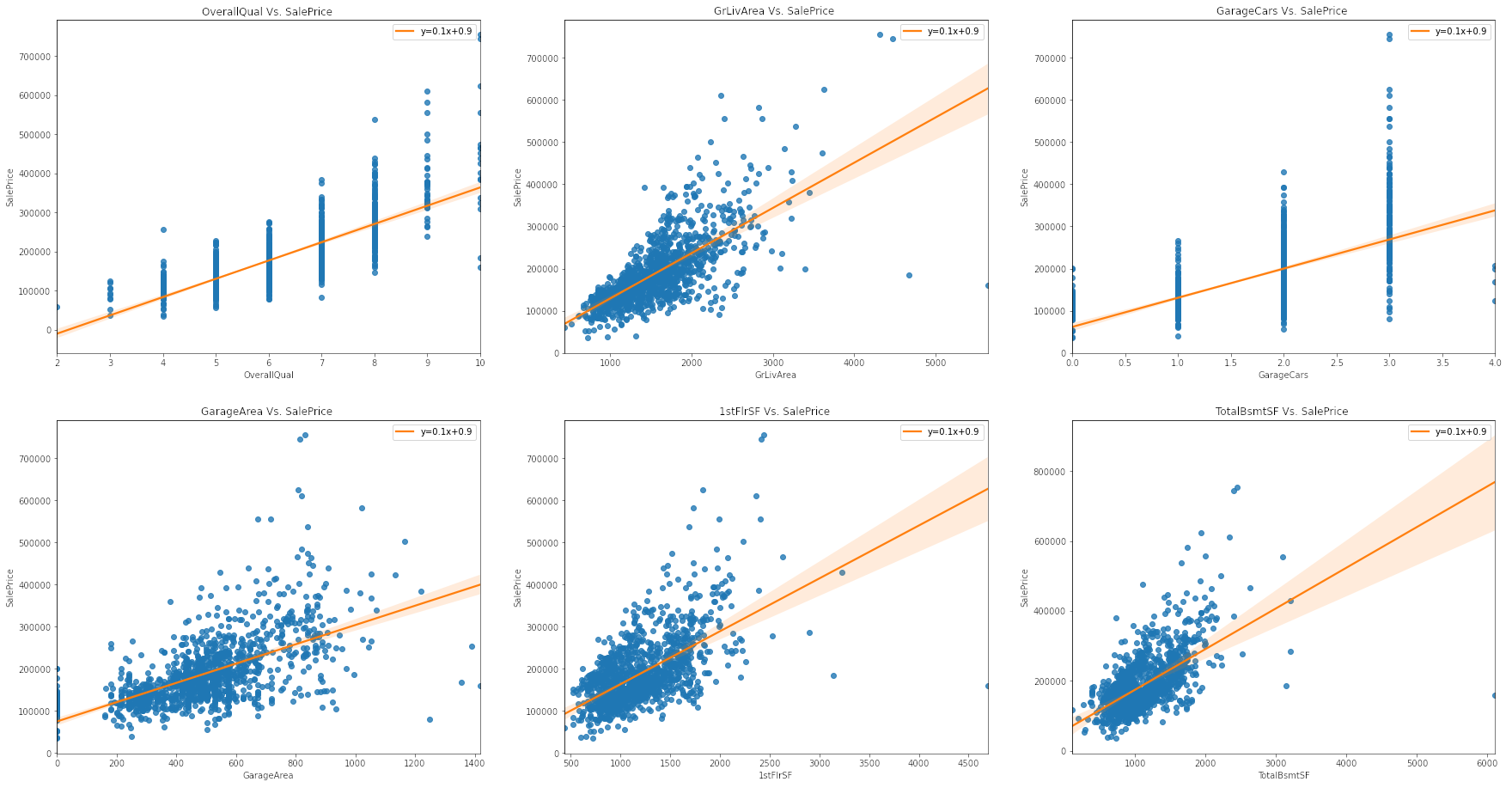
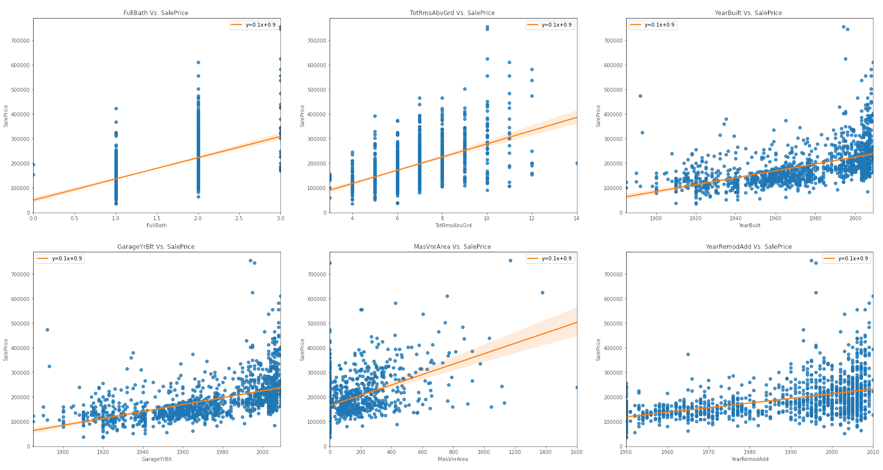
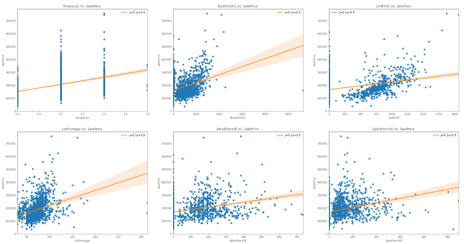
Plotting Linear Regression Between Numeric Features Vs. Target
∘ Exploring Categorial Features
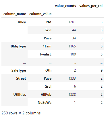
Calculating Values Count per Column
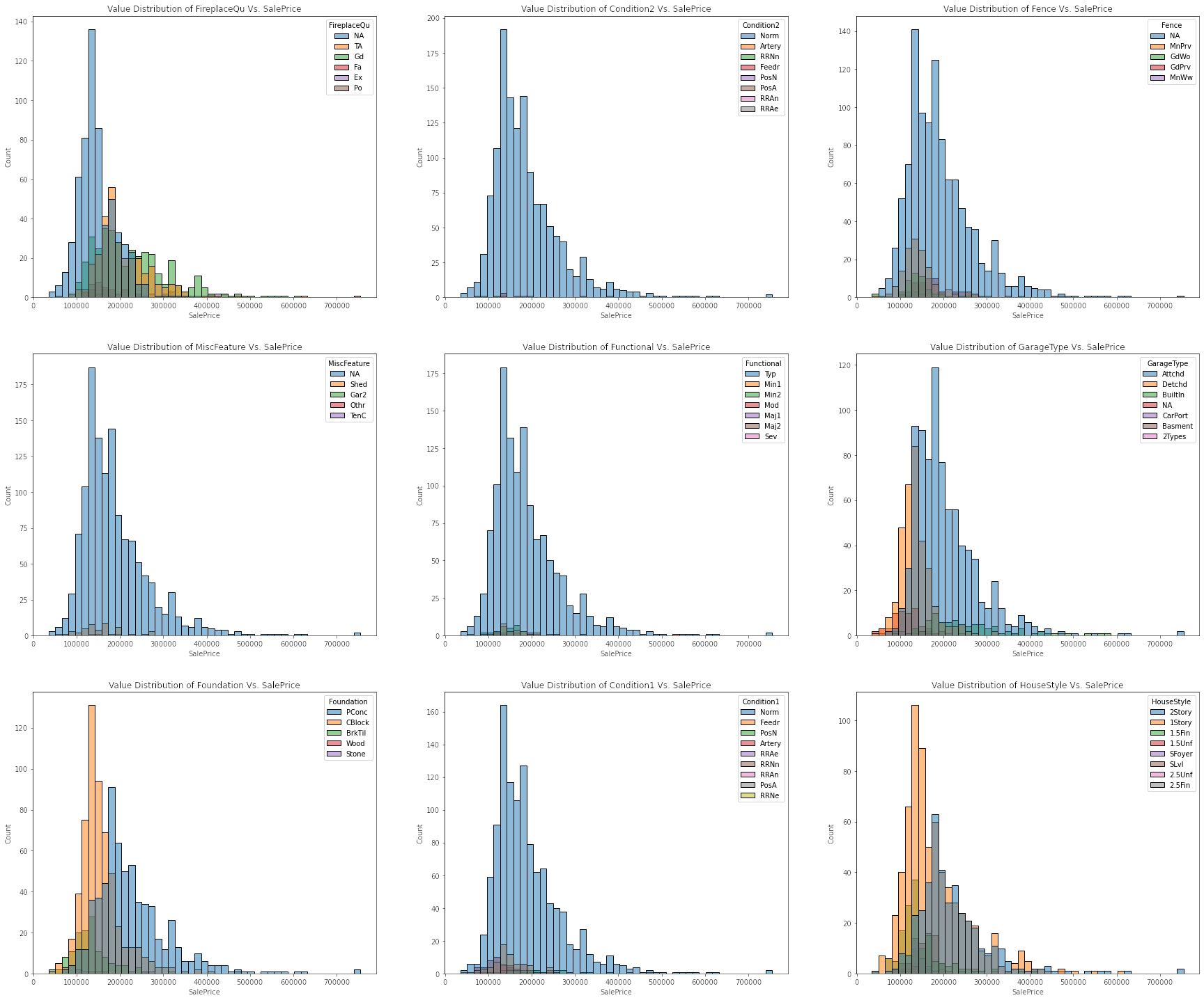
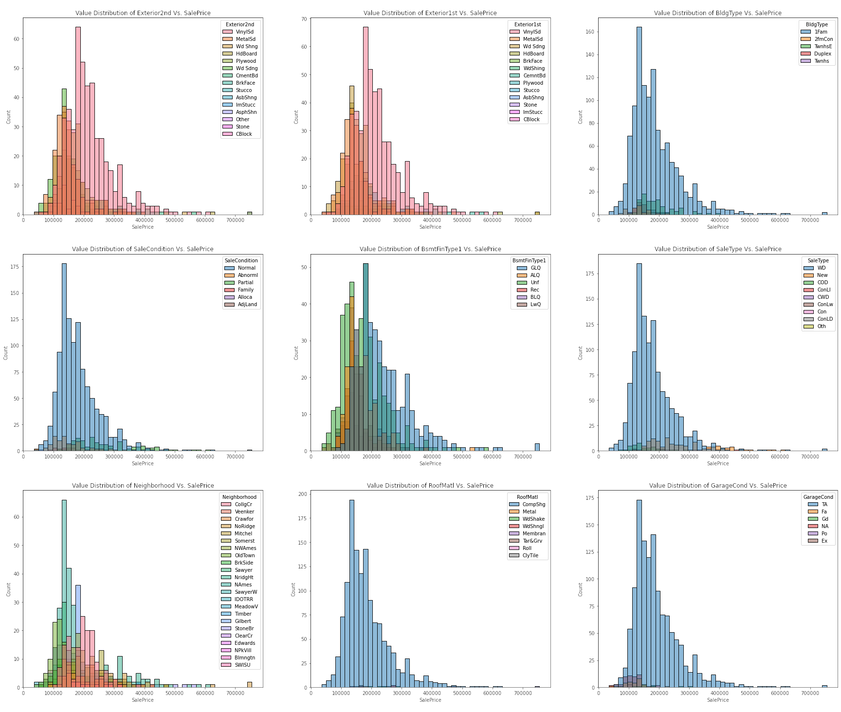
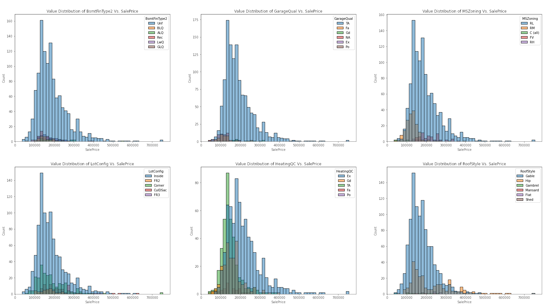
Plotting Distribution Between Categorical Features Vs. Target
∘ Graphing Correlation Between Numeric Features and Target
Correlation Between Numeric Features and Target
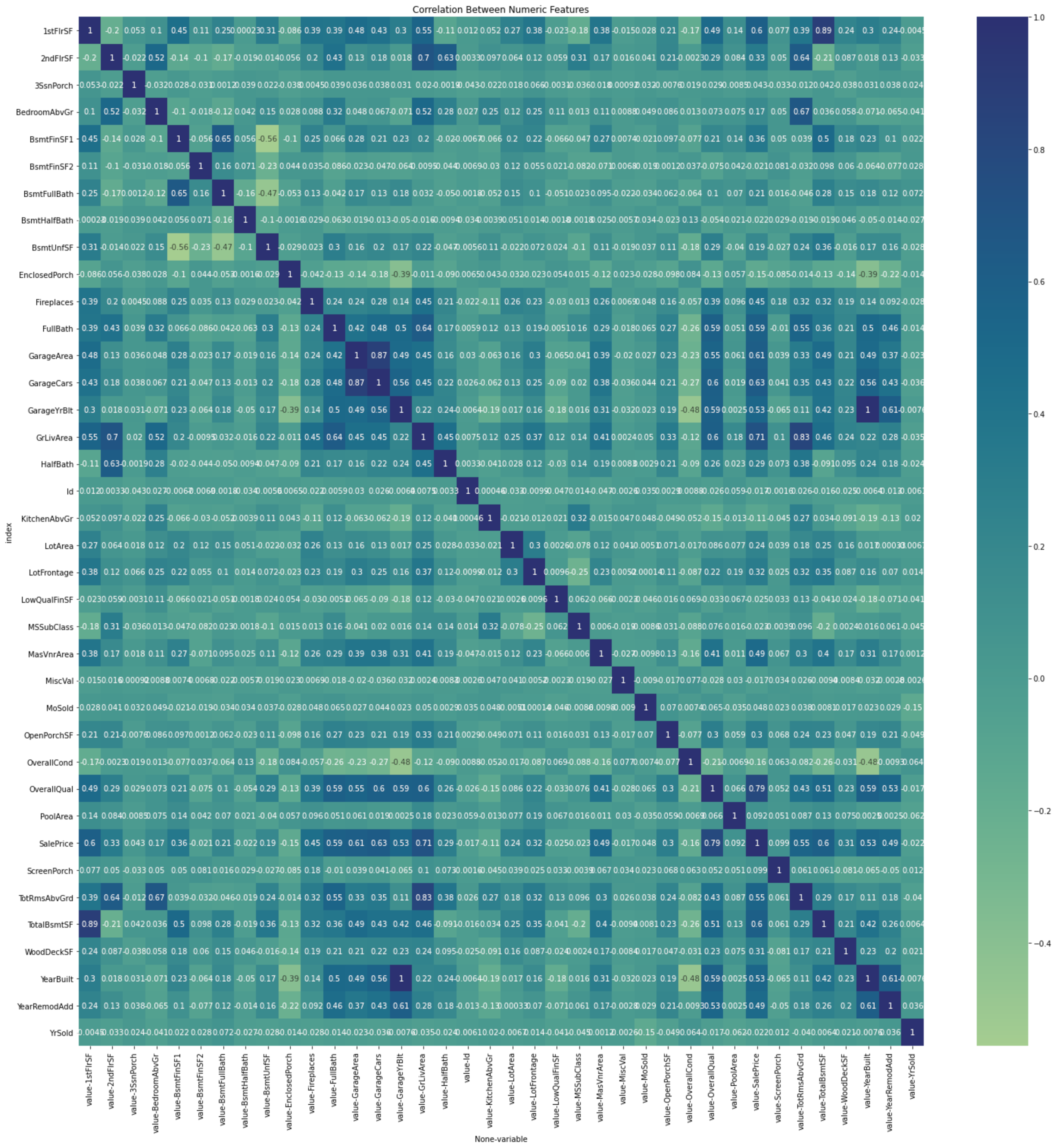
∘ Correlation Between Numeric Features
The evidence that exploring a simple linear relationship between our numeric features and target values is not a viable analysis is more apparent noting the correlation each other. First, we can observe a strong positive correlation between OverallQual vs. target values. We can also observe a similar relationship between the GrLivArea and sale price. On other hand, we can observe right-skewed distribution of FireplaceQu vs. target values, and also that of HouseType vs. sale price. Overall, the observed correlations between either type of features and the target values generally have a weak linear relationship.
∘ Transform DataFrame to Fit Our Model
As explained above, it is important that we work with a normalized distribution to ensure that we minimize any variance in our predictions. Thus, we will be applying a number of transformations according to their variable types similar to depicted above. We will be transforming our categorical variables into a series of numbers for the computer to interpret easier. Next, we will be performing the Yeo-Johnson power transformation to our more skewed numeric variables. On the other hand, we will be performing a standard scaler to our approximately symmetric numeric variables. Lastly, we will be performing a logistic transformation to our target variable. The right half of the image above depicts the transformed normalized distributions of our numeric values, which we will be using to fit our prediction model.
2. Perform Manual Parameter Tuning for Better Model Fit
∘ Define Preprocessing Transformers and Pipeline
∘ Define Each Model Parameters
The model we are fitting for this prediction model is Gradient Boosting Regressor from Scikit-Learn. The varsatility of an ensemble of forest algorithm is very impressive and handles bias and variance very well. However, we have to be very careful not to overfit the training data, which happens quite often. So, my proposed solution is to perform a very broad range of each parameter to see the effect on the predictive accuracy, and determine which combination of parameters result in underfitting or overfitting prediction model. Later, we can narrow down our combinations of parameters to a set of select few depending on the performance of our initial fitting. Finally, we will be using this smaller set of parameters to fit a more aggressive fitting to find the best estimator.
∘ Plotting Fit Performance Using RMSE Score and Percent Difference
∘ Determine Fit Performance with RMSE Score DataFrame For Better Fit
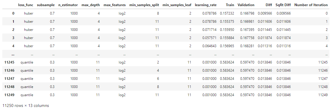
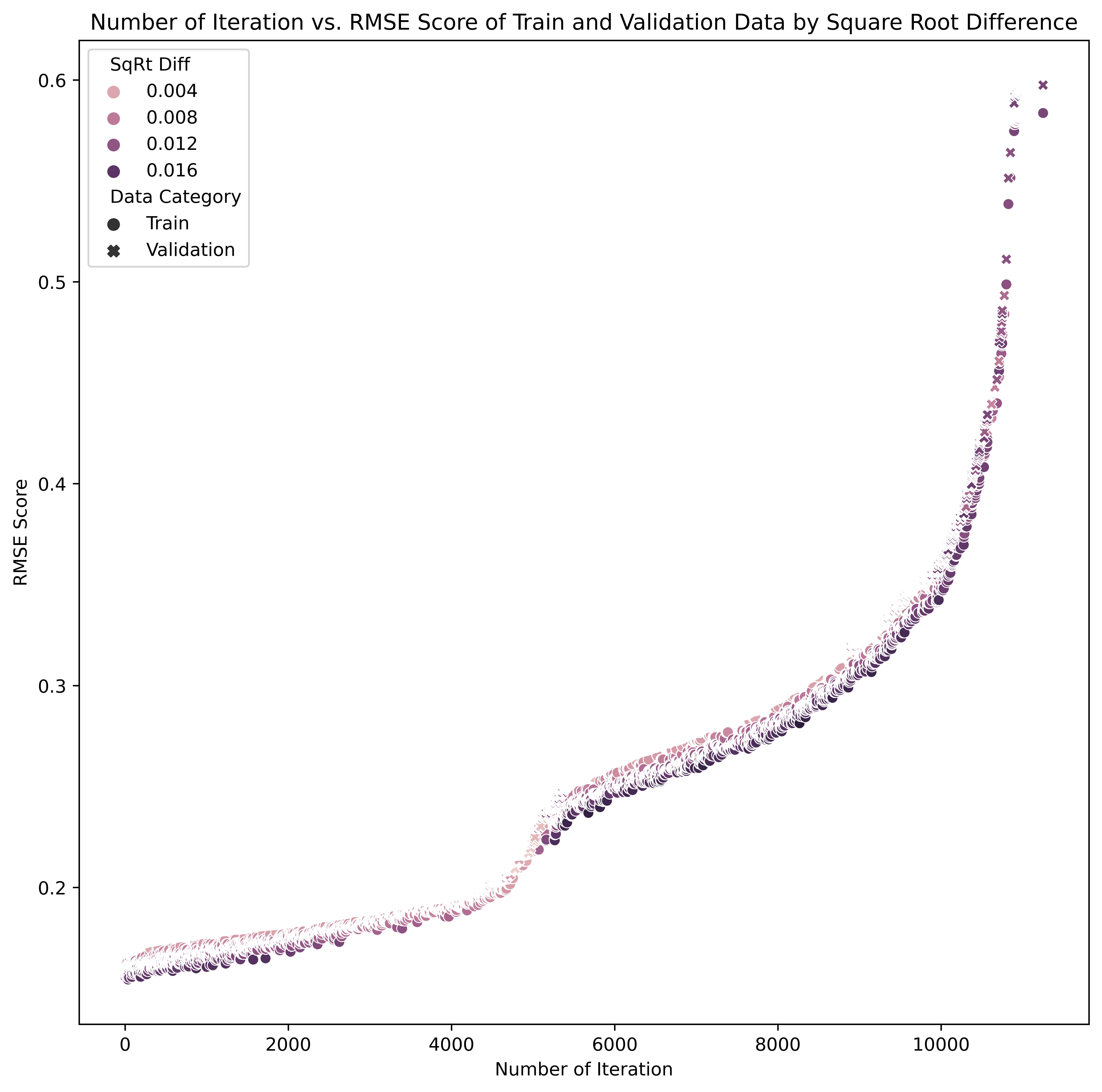
The combinations of parameters we are going to iterate are as follows: loss function types, the subsample ratio, the number of estimators, feature types, the number of depth, the number of sample split, the number of sample leaves, and learning rate ratio. In this initial parameter tuning, we are comparing the Root Mean Square Error, which is the standard deviation of the prediction errors between the training and the validation set. The range of combinations of the least square percentage difference between them will be used to fit the prediction model with the best estimator.
Here are the range of parameters in the "goldilocks zone" of bias-variance plot for this study:
- Loss Function: Huber, Quantile
- Subsample: 0.3 - 0.7
- Number of Estimators: 1000
- Maximum Number of Features: Log2
- Maximum Number of Depth: 2 - 11
- Minimum Num of Samples Split: 2 - 11
- Minimum Num of Samples Leaf: 2 ~ 11
- Learning Rate: 0.001 - 0.1
3. Improve Model Further with GridSearch and Cross-Validation Methods
∘ Define Parameters for Best Estimator
∘ Perform GridSearch Method, Model Fitting with Best Estimator, and Cross-Validate Fitting
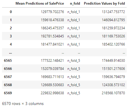
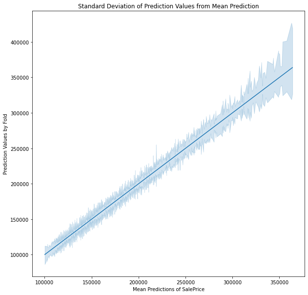
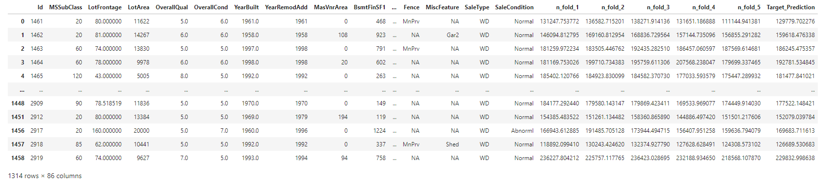
Display Girdsearch Results, Feature Importance, and Predictions
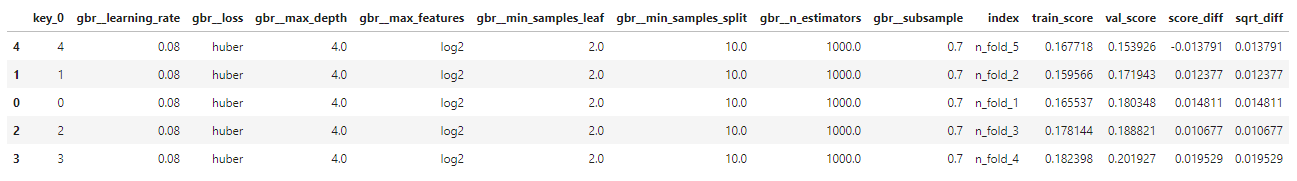
∘ Determine Fit Performance with GridSearch Best Estimator and RMSE Score DataFrame
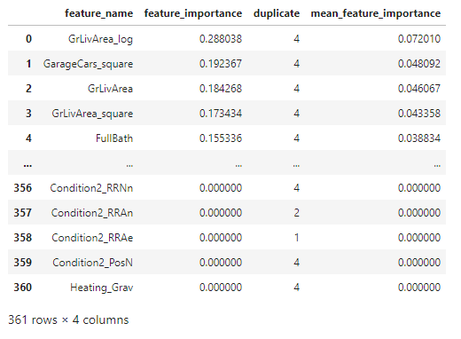
∘ Determine Feature Importance with Feature Importance DataFrame
∘ Make Predictions on Test Set DataFrame
Before fitting the model with a set of parameters, we now have a narrowed down set of parameter combinations from our initial parameter tuning. Furthermore, we will tune our prediction model with a more aggressive to find the best parameter to fit. We will be spliting our training data with shuffle split method inside and outside of the gridsearch for cross-validation. Next, we will fit the best estimator of our gradient boosting regressor model. Lastly, we score our fit and the prediction values with Root Mean Squared Error.
∘ Plotting Gradient Boosting Regressor Model Fitted with Best Estimator On A Tree Diagram
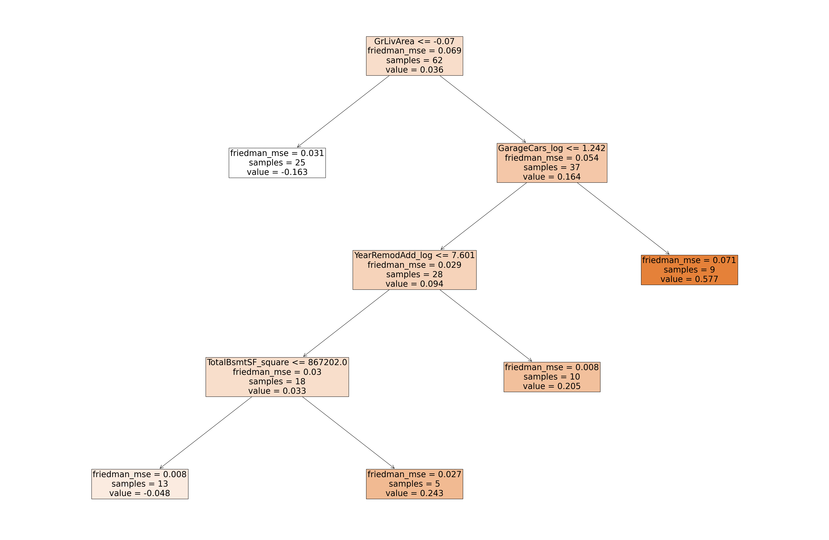
Gradient Boosting Regressor Model Diagram
∘ Plotting Tree Diagram of Grandient Bossting Regression Model
∘ Plotting Feature Importance Bar Graph
Feature Importance Bar Charts
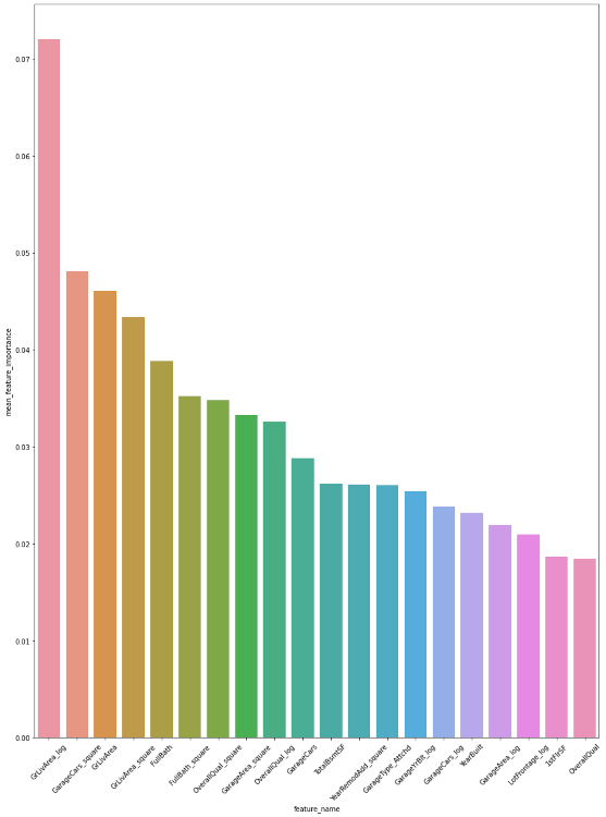
The feature importance percentage tells us that the percentage of how much the feature has the influence in our model to predict the test data. The feature with the highest feature importance is 'GrLivArea_log', followed by 'GarageCars_square', and 'GrLivArea'. However, we can note that the splitting nodes near the top of the hierarchy are 'GrLivArea', followed by 'GarageCars_log', and 'YearRemodAdd_log'. The relative position of the splitting nodes does not necessarily mean that the feature is the more important feature in a predictive model, but rather more prominent splitting feature individually. Feature importance metric tells us the overall performance of each features, which could be used to classify in multiple decisions defined by the summation of Gini importance. However, the relative position of the decision tree hierarchy tells us that the performance of a classifying feature for a single classification defined by Gini importance. Even though the feature 'GrLivArea_log' has the highest feature importance, or largest summation of Gini importance, of the entire regressor model, the feature 'GrLivArea' has the highest feature importance of an instance, or largest individual Gini importance.