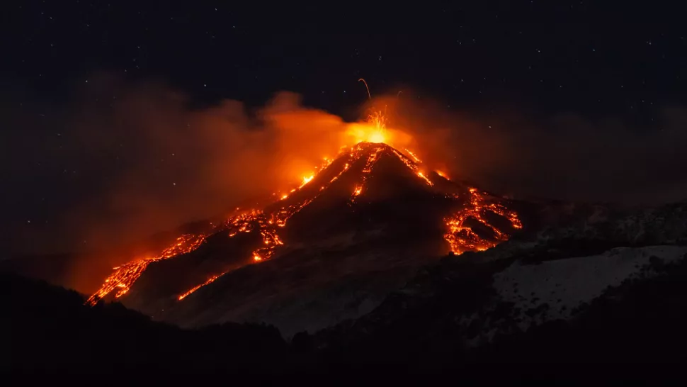
 Mount Etna, Europe's largest active volcano, spewed bubbling lava and hot as into the Sicillian sky on January 18, 2021.
(Image: © Salvatore Allegra/Anadolu Agency via Getty Images) Source: livescience.com
![]() National Institute of Geophysics and Volcanology
National Institute of Geophysics and Volcanology
What if scientists could anticipate volcanic eruptions as they predict the weather? While determining rain or shine days in advance is more difficult, weather reports become more accurate on shorter time scales. A similar approach with volcanoes could make a big impact. Just one unforeseen eruption can result in tens of thousands of lives lost. If scientists could reliably predict when a volcano will next erupt, evacuations could be more timely and the damage mitigated.
Currently, scientists often identify “time to eruption” by surveying volcanic tremors from seismic signals. In some volcanoes, this intensifies as volcanoes awaken and prepare to erupt. Unfortunately, patterns of seismicity are difficult to interpret. In very active volcanoes, current approaches predict eruptions some minutes in advance, but they usually fail at longer-term predictions.
Enter Italy's Istituto Nazionale di Geofisica e Vulcanologia (INGV), with its focus on geophysics and volcanology. The INGV's main objective is to contribute to the understanding of the Earth's system while mitigating the associated risks. Tasked with the 24-hour monitoring of seismicity and active volcano activity across the country, the INGV seeks to find the earliest detectable precursors that provide information about the timing of future volcanic eruptions.
Source: Kaggle
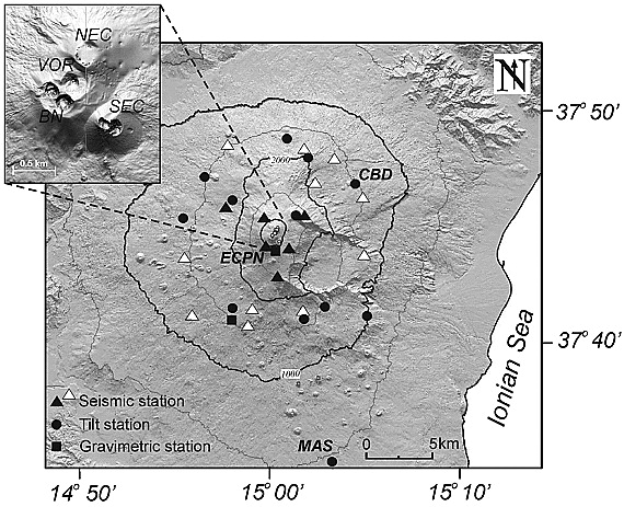 Digital elevation model of Mount Etna with seismic stations used to locate volcanic tremor (black and white triangles) and LP events (black triangles),
tiltmeters (black dots), and gravimeters (black squares) used in this work. The inset in the top left corner shows the distribution of the four summit craters
(VOR, Voragine; BN, Bocca Nuova; SEC, Southeast Crater; NEC, Northeast Crater).
Digital elevation model of Mount Etna with seismic stations used to locate volcanic tremor (black and white triangles) and LP events (black triangles),
tiltmeters (black dots), and gravimeters (black squares) used in this work. The inset in the top left corner shows the distribution of the four summit craters
(VOR, Voragine; BN, Bocca Nuova; SEC, Southeast Crater; NEC, Northeast Crater).
Source: Bonaccorso 2011
Data Description
The researchers added that detecting volcanic eruptions before they happen is an important problem that has historically proven to be a very difficult. They provided with readings from several seismic sensors around a volcano and challenged to estimate how long it will be until the next eruption. The provided data represents a classic signal processing setup that has resisted traditional methods. In addition, they commented that identifying the exact sensors may be possible but would not be in the spirit of the competition nor further the scientific objectives, and no more metadata or information that would be unavailable in a real prediction context was provided.
Assumption
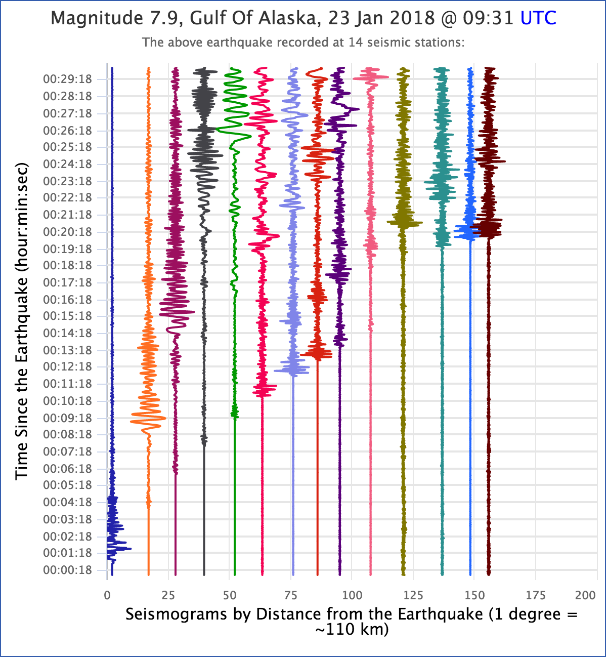
There are many observations that can be made when monitering volcanic activities. According to the United States Geological Survey, a US government agency that runs the Volcano Hazard Program, "monitoring a volcano requires scientists to use a variety of techniques that can hear and see activity inside a volcano" (Source: USGS.gov) . One of many ways to monitor the activity is seismicity, which is a technique to measure the tremor around specific locations around the earth's crust in a period of time.
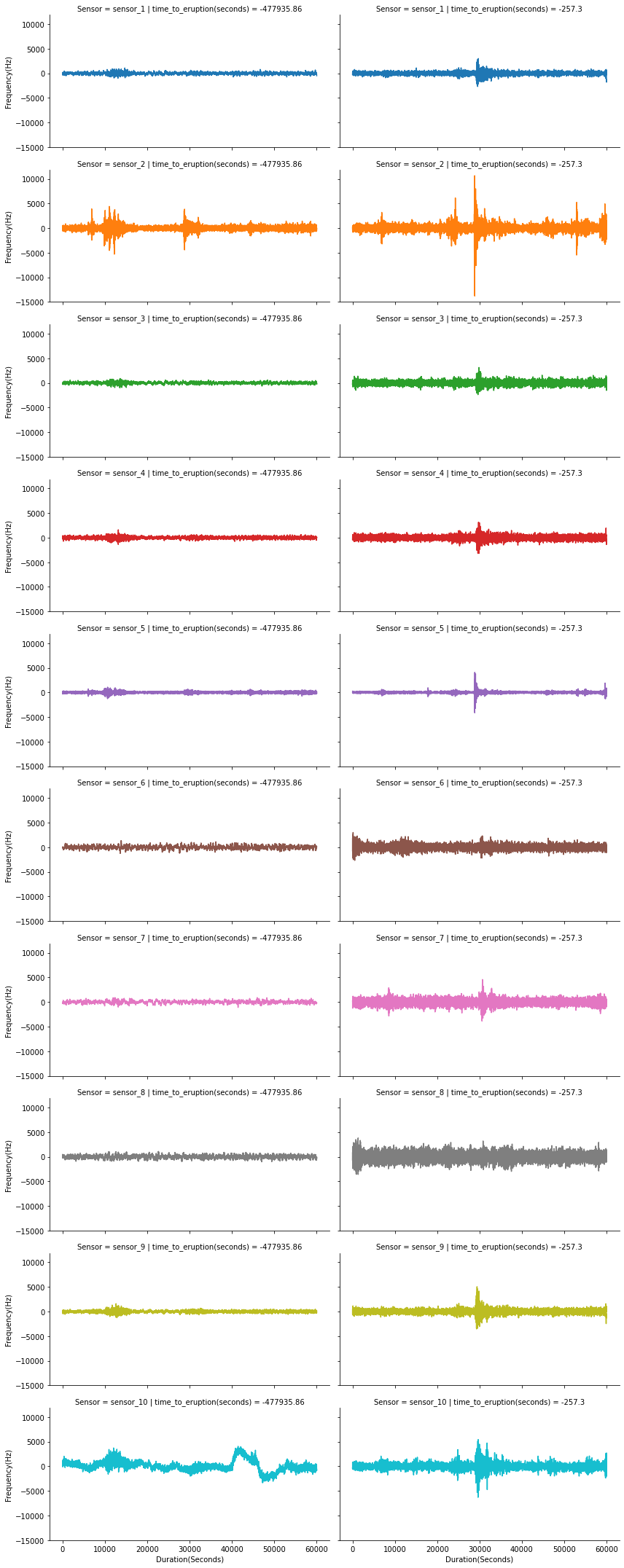
There are variety of sensor stations around Volcano Etna that measure the seismic activities of the epicenter, the tilt of the ground, and the gravity anomilies around the site. The researchers do not mention specifically what the provided data entails. However, It is safe to assume that the problem I am faced with this competition is around seismology, given that the data provided includes wide-range of frequency outputs of various undisclosed sensors around the volcano in a time-series format. I also may be wrong about my assumptions, and it is not to say that all of the provided sensor data are seismic readings. Furthermore, with my limited knowledge on volcanic seismology, I do not know why certain sensors produce different range of amplitudes and noise levels. However, I can observe changes in sensor outputs as an eruption event is imminent. As the event gets closer in time, an increase of activities is observed from a station relatively further away from the epicenter.
Goal
The goal for this study is to predict the time left until the next eruption of each seismic events by training a statistical learning model using the historical data on seismic activities at the site of Volcano Etna.
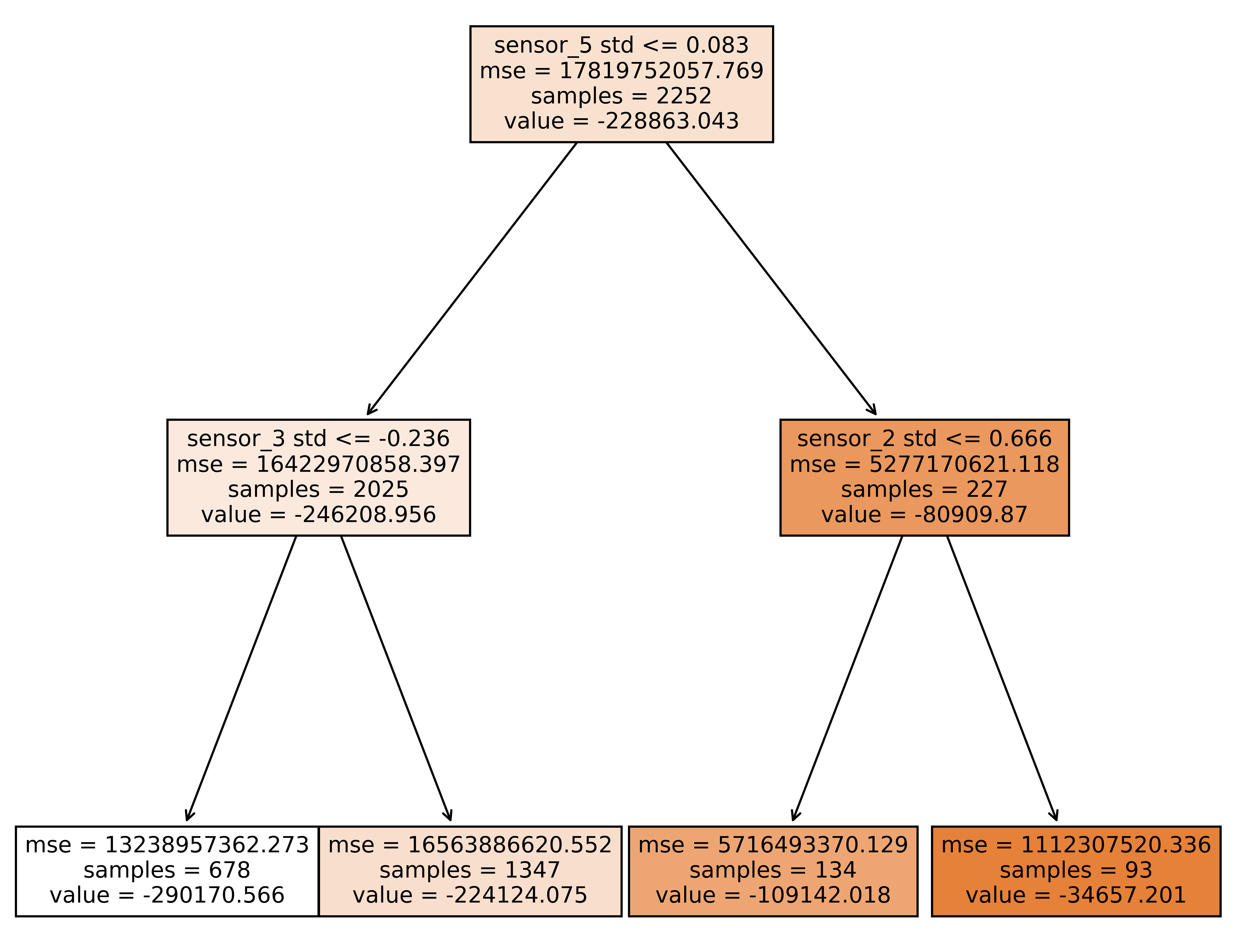
Random Forest Regressor Model Diagram
Conclusion
After analyzing the data carefully, our study concludes with predictions of each seismic reading segments in the provided test set with an error deviation of 32.95 hours until the time of eruption. By using a Random Forest Regressor method, our model is able to determine the interaction between three sensors' activities have the most infleunce on the imminent eruption event, as seen in the diagram above. More Specifically, the sensor with the most significant changes in outputs as an eruption was imminent was Sensor 5. Almost all of the sensors increased in noise levels as the event was getting closer in time. However, Sensor 5 have stayed almost to the same level, up until the last 5 minutes to the event, which we can explore with a time-series chart along with a series of histograms. By training our machine learning model with the provided test data, we can estimate that we can predict the next volcanic eruption about 3-4 days prior.
Walkthrough
∘ Define Data Path
∘ Import Libraries
∘ Define Custom Functions
∘ Define Plotting Functions
∘ Perform Data Acquisition and Preparation
1. Define DataFrames, Features and Target
train.csv Metadata for the train files.
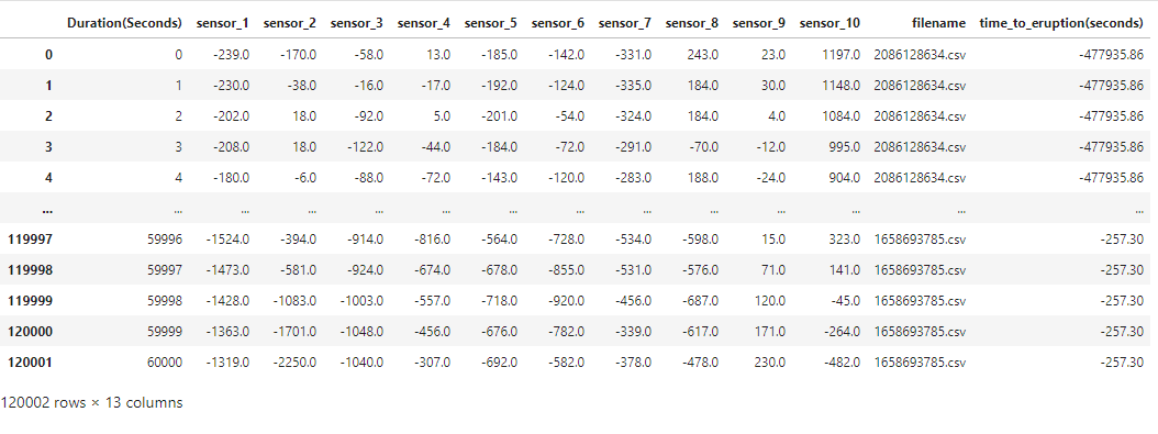
[train|test]/*.csv: the data files. Each file contains ten minutes of logs from ten different sensors arrayed around a volcano. The readings have been normalized within each segment, in part to ensure that the readings fall within the range of int16 values.
∘ Prepare DataFrame to Fit Our Model
∘ Retrieve Original Sample DataFrame
∘ Transform Train DataFrame
∘ Transform Test DataFrame
∘ Sample Sensor Outputs(Hz) Compared with Time To Eruption (seconds) Plot
Segment Duration (Seconds) Vs. Sensor Outputs(Hz)
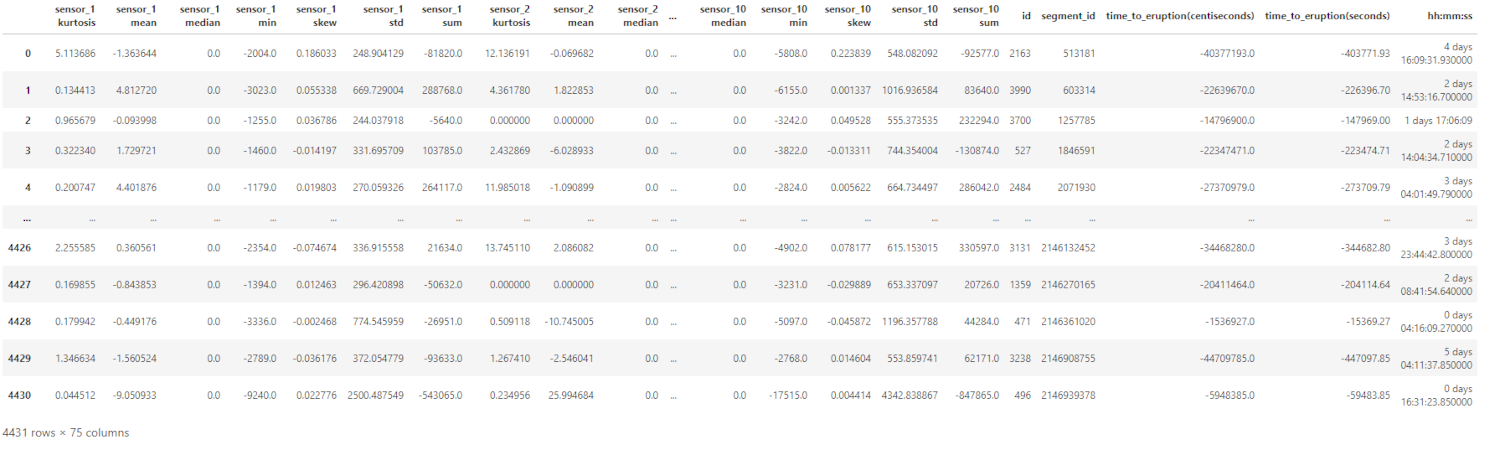
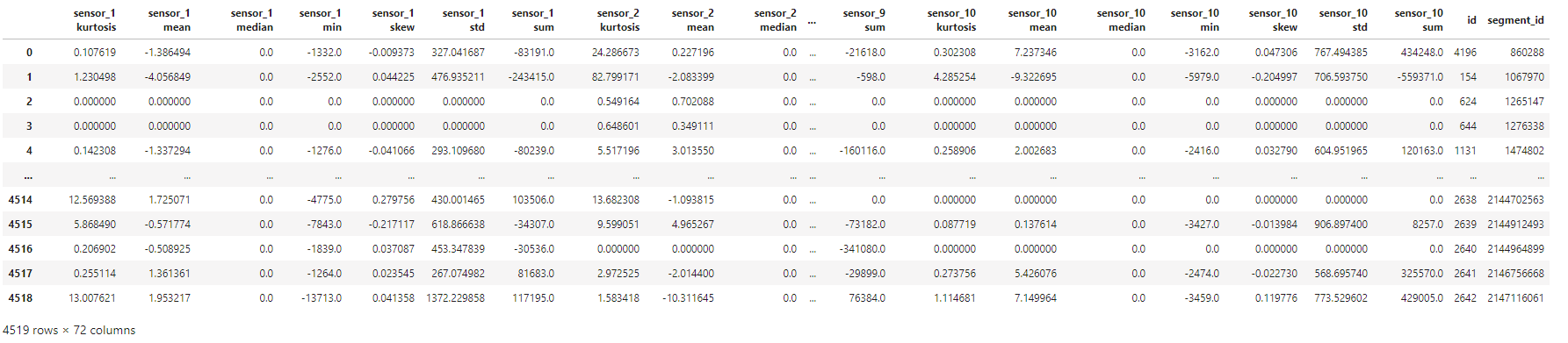
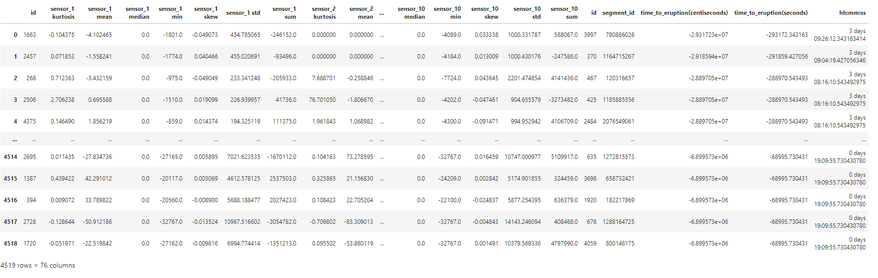
To be more specific, each segment contains 10 minute long sequence of 600,001 sensor readings. The training data file includes 4,431 segments. The total sensor readings in the training file come out to be over 2.6 million sequences for each 10 sensors reading. Also, the test data file includes 4,520 segments. The total sensor readings in the prediction file comes out to be over 2.7 million sequences for each 10 sensors reading. Because of the shear size of the dataset, we can explore the aggregation of different statistical descriptions of each segment per sensor to work with an overview of the distribution. These descriptions include the sum, minimum, mean, standard deviation, median, skewness, and kurtosis. Thus, the feature names of our machine learning model are the statistical descriptions of each sensors. Also, this will reduce the size of our working dataset to improve its workability. The target is the time to eruption measured in seconds. The result dataframe is callable by the functions defined above.
2. Perform Manual Parameter Tuning for Better Model Fit
The model we are fitting for this prediction model is Random Forest Regressor from Scikit-Learn. The varsatility of an ensemble of forest algorithm is very impressive and handles bias and variance very well. However, we have to be very careful not to overfit the training data, which happens quite often. So, my proposed solution is to perform a very broad range of each parameter to see the effect on the predictive accuracy, and determine which combination of parameters result in underfitting or overfitting prediction model. Later, we can narrow down our combinations of parameters to a set of select few depending on the performance of our initial fitting. Finally, we will be using this smaller set of parameters to fit a more aggressive fitting to find the best estimator.
∘ Define Pipeline
∘ Define Each Model Parameters
∘ Determine Fit Performance Metric and Perform Manual Parameter Tuning for Better Fit
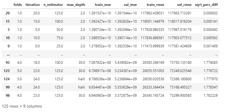
∘ Determine Fit Performance with RMSE DataFrame For Better Fit
∘ Plotting Fit Performance Using RMSE Score and Percent Difference
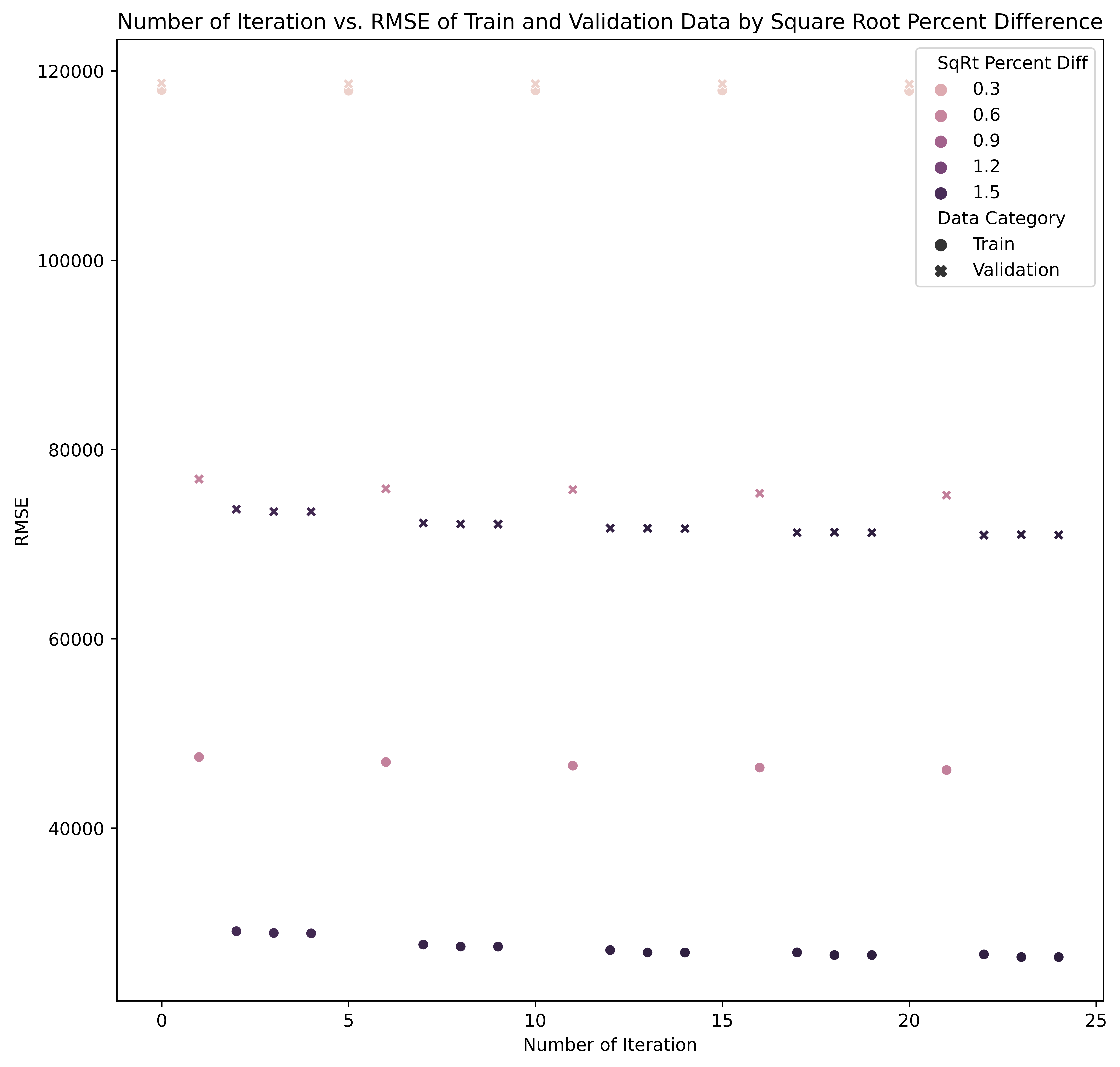
The combinations of parameters we are going to iterate are as follows: the number of estimators, and the number of depth. In this initial parameter tuning, we are comparing the Root Mean Square Error, which is the standard deviation of the prediction errors between the training and the validation set. The range of combinations of the least square percentage difference between them will be used to fit the prediction model with the best estimator.
Here are the range of parameters in the "goldilocks zone" of bias-variance plot for this study:
- N Estimators: 25 ~ 125
- Max Depth: 2
3. Improve Model Further with GridSearch and Cross-Validation Methods
Before fitting the model with a set of parameters, we now have a narrowed down set of parameter combinations from our initial parameter tuning. Furthermore, we will tune our prediction model with a more aggressive to find the best parameter to fit. We will be spliting our training data with shuffle split method inside and outside of the gridsearch for cross-validation. Next, we will fit the best estimator of our gradient boosting regressor model. Lastly, we score our fit and the prediction values with Root Mean Squared Error.
∘ Define Parameters for Best Estimator
∘ Perform GridSearch Method, Model Fitting with Best Estimator, and Cross-Validate Fitting
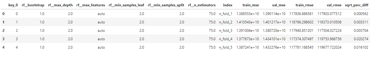
∘ Determine Fit Performance with GridSearch Best Estimator and RMSE DataFrame
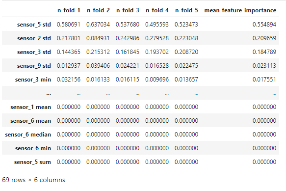
∘ Determine Feature Importance with Feature Importance DataFrame
∘ Make Predictions on Test Set DataFrame
∘ Plotting Our Random Forest Regressor Model Fitted with Best Estimator On A Tree Diagram
Random Forest Regressor Model Diagram
∘ Plotting Feature Importance Determined by Our Model on a Box Plot
Random Forest Feature Importance
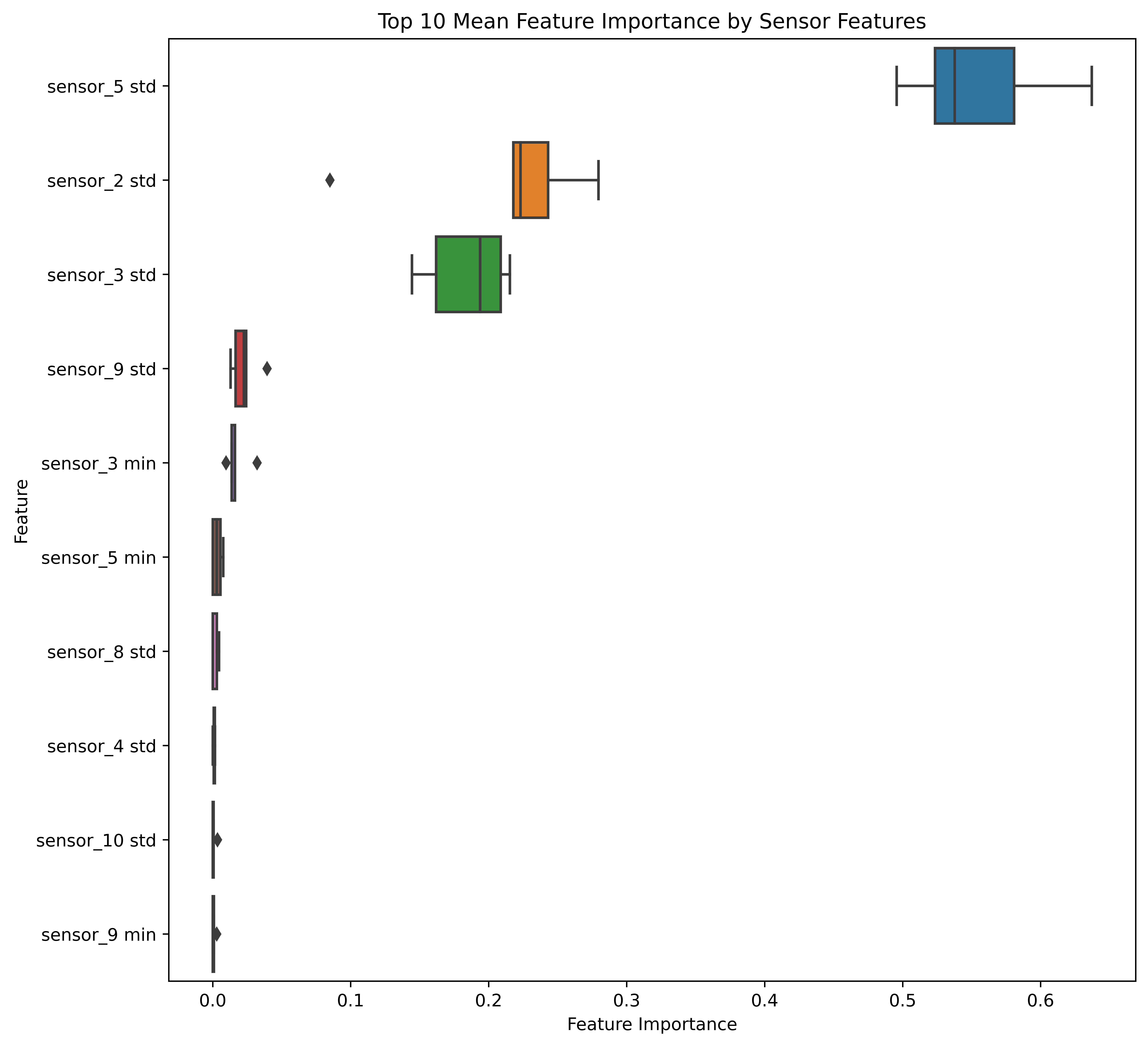
;The feature importance percentage tells us that the percentage of how much the feature has the influence in our model to predict the test data. Out of the 70 features, which is comprised of aggregation of 7 statistical description of 10 sensors, the most important feature of this model is the standard deviation of Sensor 5. In this study, we conclude that our most influential feature takes account of 55% of decisions to predict the test data. The next most influential features include the standard deviation of Sensor 2 with 21% of influence, and that of Sensor 3 with 18% of feature importance.
∘ Plotting Most Influential Sensor Outputs On A Time-Series Chart
Top 5 Most Influential Sensors Outputs Based On Training Data
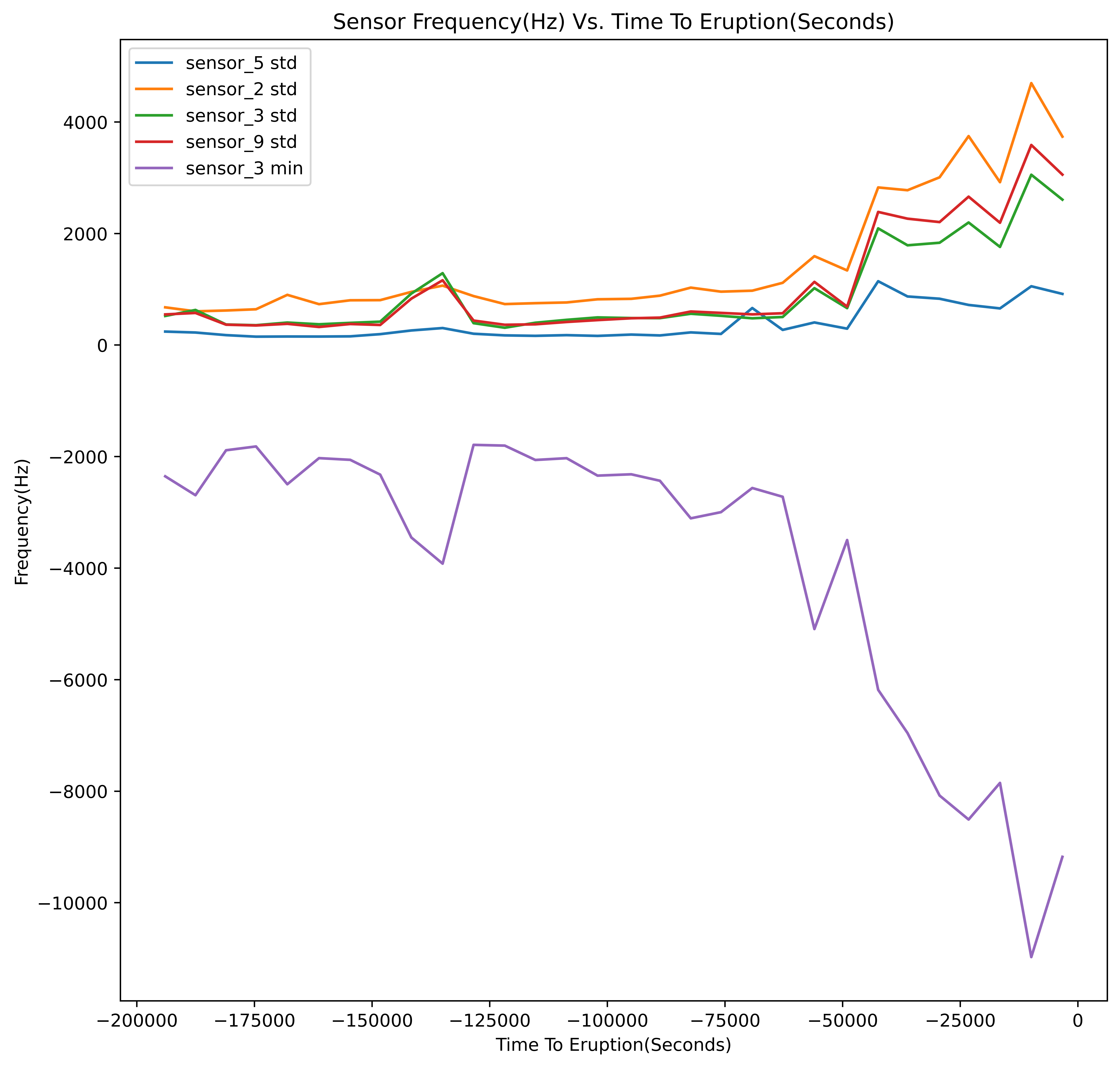
Top 5 Most Influential Sensors Outputs Based On Prediction Data
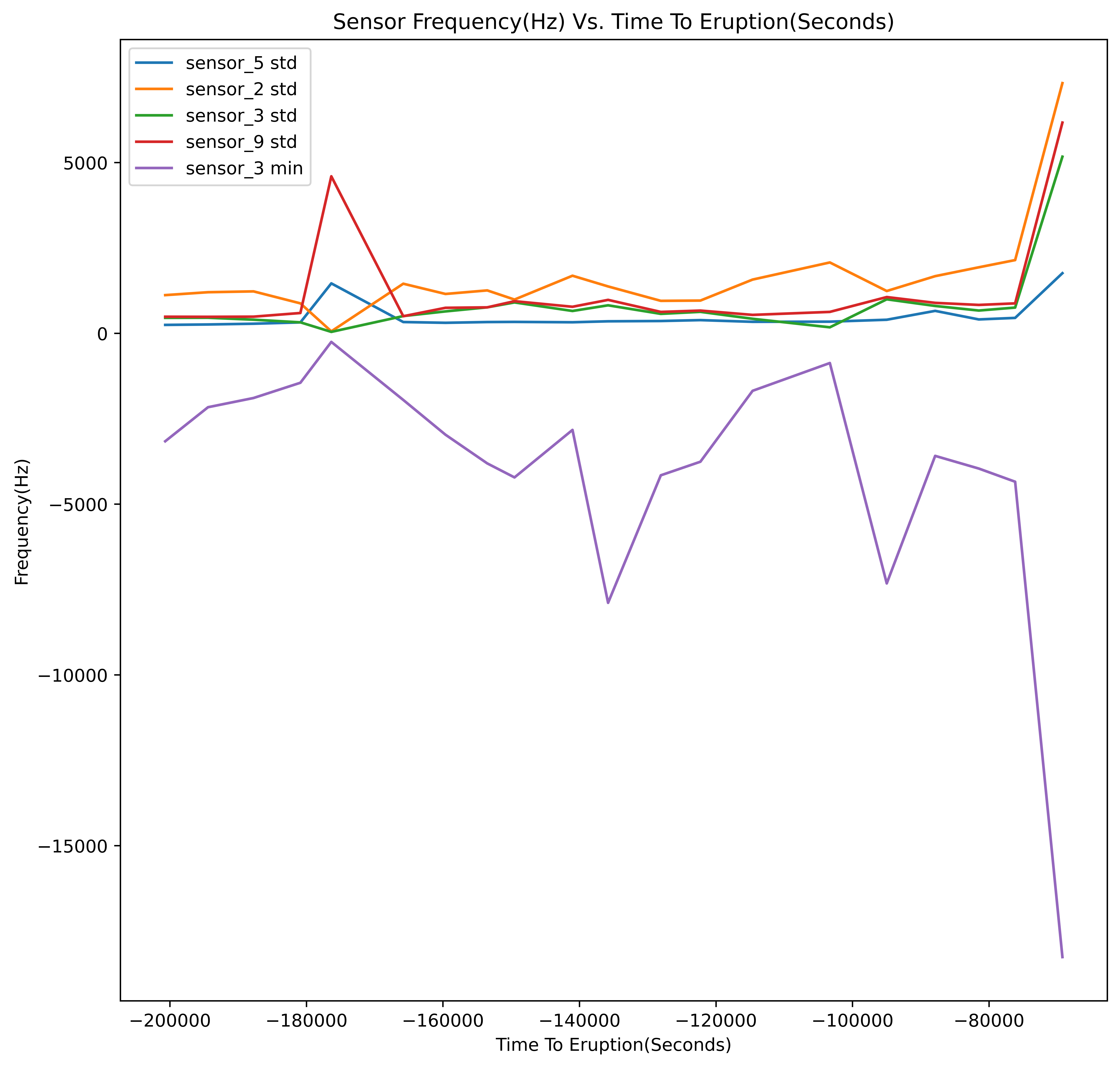
The above image is the time-series graph of top 5 most influential sensors. We can observe that the most influential features actually do not have significant changes over time, which might have many confused. In fact, they seem to have the least amount of changes over time in this graph. Consequently, the feature with the most change over time is the minimum values of Sensor 3, which the least important feature out of these 5 features.
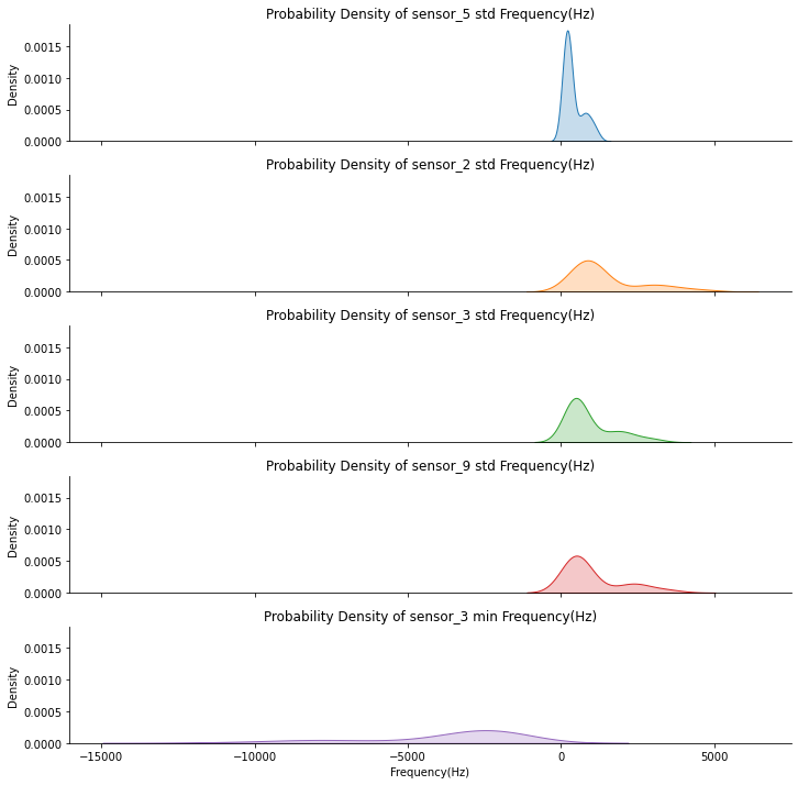
∘ Plotting Sensor Output Distributions of Top 5 Most Influential Sensors On A Ridgeline chart
Top 5 Most Influential Sensors Outputs Based On Training Data
Top 5 Most Influential Sensors Outputs Based On Prediction Data
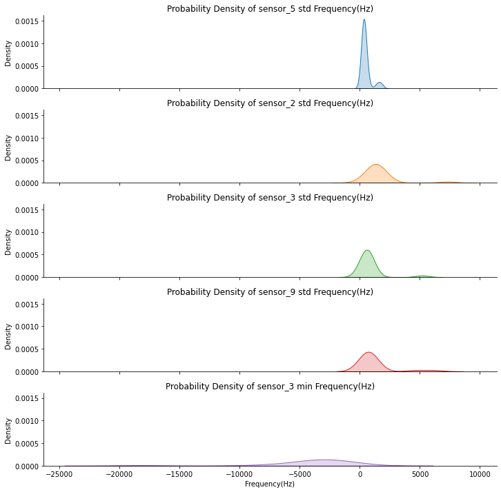
However, the probability density, more specifically the tail-heaviness characteristics, of these 5 features is consistant in conveying the features' infuence on our predictive model. The differences in kurtosis, which is the measure of the combined weight of the tails relative to the rest of the distribution, of these 5 features gives us an idea of the sensitivity of each sensors to earth's tremor during a dormant period, and a period leading up to an eruption event. We can observe that features that have lesser influence on the model decisions tends to have a relatively lower peak of the value density. This suggests that lower the peak, heavier the distribution is at the tails, more sensitive the readings are to earth's tremor, and have relatively higher in noise levels even in dormant periods. Thus, they may seem to have the most significant changes over time on a time-series chart, but the distribution suggests that such extreme readings are still present during a dormant period, and amplifies as an eruption event is imminent. Conversely, the feature with the most influence, Sensor 5, stays very quiet throughout the period until the last several minutes before the big event occurs, making it the sensor that is least sensitive to normal earth's tremor.